Transport of Molecules in Solution

Modes of Transport

There are three possible ways that molecular transport occurs in an electrolyte solution; migration, convection, and diffusion. Convection is the movement of molecules in solution due to random thermal currents. Convection is sometimes useful and can be purposefully invoked using a stirbar or a rotating electrode setup, but for our purposes it is undesirable and solutions should remain undisturbed at all times during the experiment.

Migration is the movement of molecules due to a charge gradient. Migration is the means through which current is conducted through solution. When a negatively charged species is generated at a negatively polarized electrode, it “migrates” toward the positively charged electrode. We minimize migration by including supporting electrolyte at a high concentration. By having an excess of other charged species in solution, the analyte does not feel the tendency to migrate.

Diffusion is the only mode of analyte transport (or “mass transport”) that we care about in a homogeneous CV. Diffusion is the tendency for a species in solution to move from an area of high concentration of the species to an area with a lower concentration. When a species is continually generated at an electrode, it begins to diffuse away from the electrode, where its concentration is zero. Similarly, when an analyte is consumed (when X is reduced to X^–), its concentration near the electrode decreases and more analyte diffuses in from further away to replenish it. The rate of diffusion increases with increasing concentration gradients (steeper slopes). In the same way that air moves fastest between areas of high pressure gradients and a ball will roll fastest down a hill with the highest potential energy gradient (steepest slope), molecules will diffuse the fastest when the concentration gradient is highest.

Concentration Gradients and Observed Current

As the potential changes during a CV, electrons are transferred, concentrations change, and diffusion occurs. All of these factors must be understood at a qualitative level in order to interpret CVs while they are being collected. Let us remember that the line that traces the outline of the waves we see in a CV is a measure of current passed as the electrode potential changes. Current is a measure of electrons passed per unit time. In a reversible wave, the amount of current registered depends on how much X can approach the electrode per unit time, which is determined by the rate of diffusion and therefore the concentration gradient near the electrode. We will reinforce this point and explain the shape of a CV wave by creating a concentration vs. distance graph for each position that we outlined in the previous section about the Nernst equation.

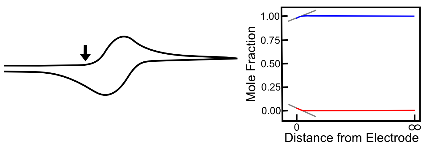
When the electrode potential is far positive of the X/X^– reduction potential, the concentration close to the electrode is essentially the same as it is in the bulk solution. The concentration gradient is effectively zero, so there is no net movement of analyte in any particular direction. Note that in the graphs below, the blue line represents the concentration of X, and the red line that of X^–, as the distance from the electrode increases.

As the potential approaches the foot of the wave, a small amount of X is converted to X^–, but the mole fraction of X only a short distance away from the electrode remains at near 1 (100%). Nevertheless, there is a small concentration gradient that is formed, which causes some X to diffuse toward the electrode. The graph below shows the concentration gradients of X and X^– for the example that we worked out in the previous section where there the mole fraction of X^– at the electrode is 0.01 (1%). Gray lines with slopes representing the concentration gradient of X and X^– has been added to the graphs below to demonstrate its relation to the current registered by the potentiostat.

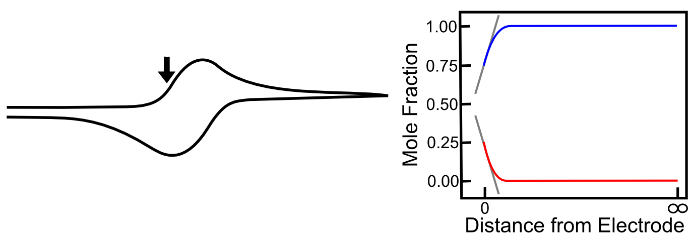
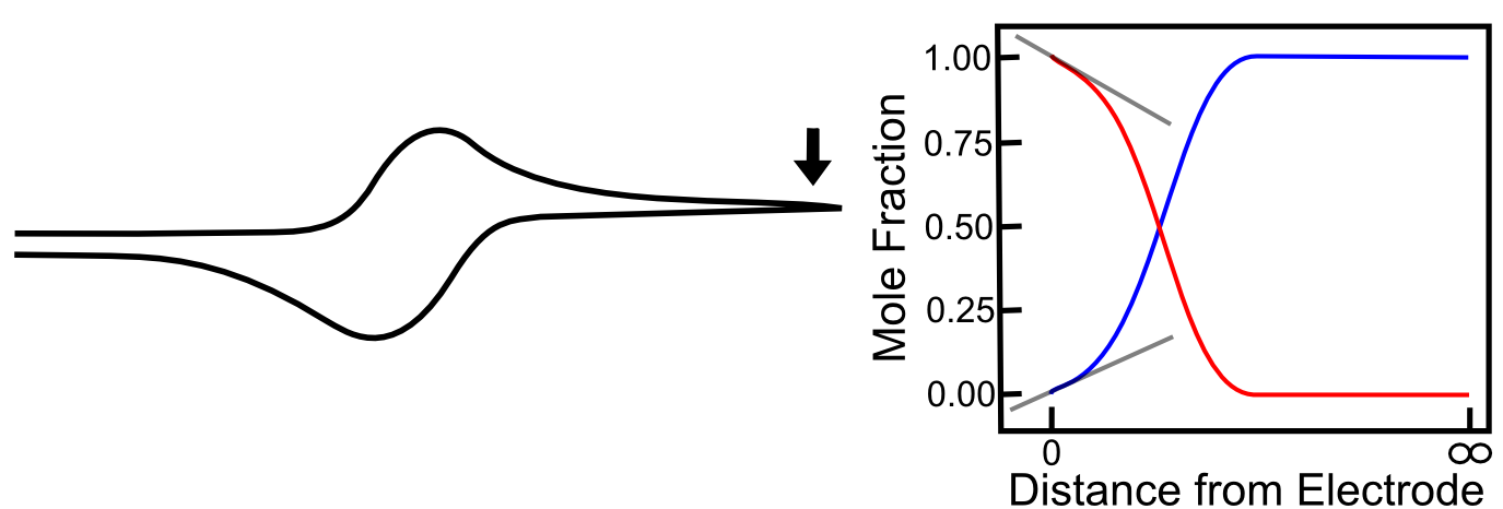
As the potential continues to scan to more negative values, the concentration of X^– at the electrode increases, and the concentration of X at the electrode decreases, and the concentration gradients (the slope of the red and blue lines near the electrode) get steeper, meaning that diffusion occurs more rapidly than before and the current continues to rise. The graph below includes the corresponding concentration gradients for the example from the last section where the mole fraction of X^– is 0.25 (25%).

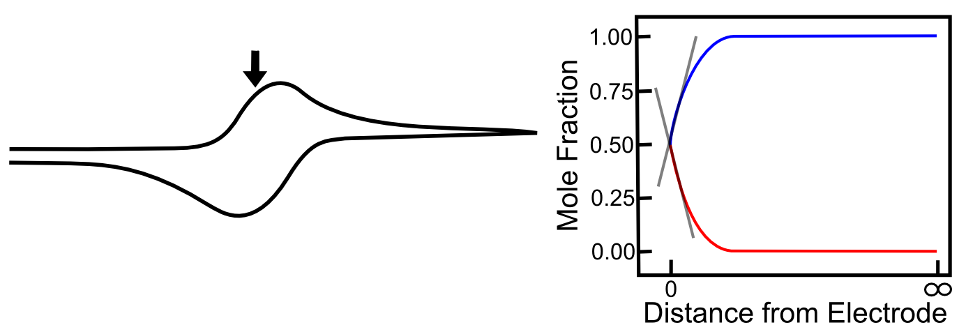
When the electrode potential reaches the E_1/2, the concentrations of X and X^– are equal at the electrode. The slopes of the red and blue lines are as steep as they have been so far in the scan, but they are not as steep as they could be. In other words, X is not moving toward the electrode as fast as it can, therefore the number of electrons transferred at any given time (current) could be higher, becuase the concentration gradient is not as high as it can be. Similarly, X^– is not diffusing away from the electrode as fast as it could be for the same reason. This is why current is not at a maximum yet.

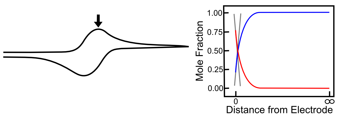
As we travel a further distance away from E_1/2, there is significantly more X than X^–, but more importantly, the slopes of the red and blue lines continues to get steeper until they reach a maximum at 29.5 mV more negative than the E_1/2. Diffusion is occurring as fast as it can, new X is appearing at the electrode at a high rate, which allows the maximum rate of electron flow (current) to occur. At the E_p (peak potential), we have the maximum slope of the concentrations of X and X^– near the electrode, and this is the reason we see the maximum current here.

As the scan continues, the concentration of X far away from the electrode starts to decrease (as more is depleted after diffusing to the electrode) and the concentration of X^– far away from the electrode begins to increase (as the X^– produced at the electrode begins to diffuse into solution). This causes the concentration gradients to decrease (the slopes of the red and blue lines above flatten) which lower rates of diffusion and an overall decrease in current. When the potential has far surpassed E⁰(X/X^–), the concentration gradients settle to a steady state value, which is the reason we see the current converge to the value we call the “limiting current,” also known as the "diffusion limited current."

On the return sweep, the reverse reactions happen and the same, but opposite concentration gradients occur near the electrode, giving rise to the familiar reversible wave. Putting all these pictures together, we can see a crude animation of the concentrations of X and X^– near the electrode throughout the course of a potential sweep.

The Absence of Diffusion

To illustrate the role that diffusion plays in the shape of a reversible wave, we can look at the case where the analyte X is attached to an electrode surface, which can be done in a variety of ways. Assuming the X/X^– reduction is still electrochemically reversible, the ratio of X to X^– at the surface will still be determined by the Nernst equation, but after a molecule of X has been converted to X^–, it sticks around, and no more X can come in to replenish it. Current rises until it reaches the E_1/2 of the X/X^– couple. Up to this point, electrons could be transferred to an increasing number of molecules of X in order to maintain the ratios of X to X^–, but after E_1/2, there is a decreasing number of unreduced X molecules available, so current decreases. In this case, the E_p (peak potential) is the E_1/2!

hover over pic for description

• Previous Section - The Nernst Equation
• Next Section - Ion Pairing